aw.stats

In this time of the pandemic I feel completely overwhelmed by the information available via the news, on the internet or thrown at me in lots of different conversations. Trying to take in every single piece of data and contextualize it quickly became impossible especially that when you couple it with work. Originally I felt compelled to try my hand at mapping spreads, infection rates and various other pieces but immediately felt out of my depth in subject matter and took to spreading the high quality information from those that were experts.

Quite a few months in now and I find myself wanting, as I usually do, to use data to understand. The issue was still finding data that I felt answered questions I had. Enter YouGov which is a global data and survey company that has supplied loads of different data I have used in the past. Recently YouGov partnered with the Institute of Global Health Innovation (IGHI) at Imperial College London to gather global insights on people’s behaviours in response to COVID-19.

It is designed to provide behavioural analysis on how different populations are responding to the pandemic, helping public health bodies in their efforts to limit the impact of the disease. Anonymised respondent level data will be available for all public health and academic institutions globally. The questions in the survey, led by IGHI, cover data on testing, symptoms, self-isolating in response to symptoms and the ability and willingness to self-isolate if needed. It also looks at behaviours, including going outdoors, working outside the home, contact with others, hand washing and the extent of compliance with 20 common preventative measures. -IGHI Data Tracker website

This data is super rich and I have only just scratched the surface. The data seemed to have the answers to some of the questions I was asking myself:

Are people wearing masks?
Are people using public transit?
Are people avoiding small gatherings?

These questions to me are interesting on their own but it is my hope that this data will help me explore the intersection of this data. But I don’t want to get ahead of myself, so this post is mostly to provide a jumping off point for how to interact with this data and visualize the responses.

Data & Information

Imperial College London YouGov Covid 19 Behaviour Tracker Data Hub
The IGHI has built a publicly available dashboard to visualise the data if you are interested also.

code

First you should download a copy of the data folder from the repository above and set your working directory to that file location.

library(tidyverse)
library(awtools) #just for plot aesthetics, not necessary
library(viridis)

temp <- list.files(pattern="*.csv")
tempfilenames <- temp %>% as.list()
templist <- lapply(temp, read.csv)

After loading the packages we create a list of the CSV files in the location, create a list of the names to use later and load in the data. Within the repository on Github there is a ‘codebook’ file that provides details on the fields included, I found the fields that pertain to the questions I was interested in and grabbed those. I then select only those fields and add the filename to the lists to identify the country the results are from. The rest is massaging the data into a cleaner form.

#cols
ivars <- c('i12_health_1','i12_health_8','i12_health_12') #wore a mask, avoided public transport, avoided small gatherings, government Response
tempvars <- lapply(templist, function(x) x[(names(x) %in% ivars)])
tempvars <- mapply(c, tempvars, tempfilenames, SIMPLIFY = FALSE)

#dataframe
tracker_files <- data.frame(do.call(rbind, tempvars),stringsAsFactors = FALSE)
tracker_data <- tracker_files %>% unnest(cols = c(i12_health_1, i12_health_8, i12_health_12, V4))

#Massage data
raw_data <- tracker_data %>%
  transmute(mask=`i12_health_1`,
            transport=`i12_health_8`,
            gathering=`i12_health_12`,
            country=V4) %>%
  mutate(country=str_to_title(str_extract(country, '^[^.]+')))

Once that is done I create (in a very stream of consciousness way) a summary dataframe and a dataframe of data for ordering on the ‘Always’ response and join it all together to get ready to plot.

covid_data <- raw_data %>%
  group_by(country) %>%
  gather('variable','Response',1:3) %>%
  ungroup() %>%
  group_by(country, variable, Response) %>%
  tally() %>%
  ungroup()

ord_data <- covid_data %>%
  group_by(country,variable) %>%
  mutate(total=sum(n)) %>%
  filter(Response=='Always') %>%
  mutate(order=n/total) %>%
  select(-c(3:4))

covid_data <- covid_data %>% left_join(.,ord_data)

With survey data I usually like to see the data as a percent stacked bar chart so we will create three of those, one for each of the questions.

covid_data %>%
  filter(variable == 'mask',
         Response != ' ') %>%
ggplot(., aes(x = reorder(country,order), y = n, fill = Response)) + 
  geom_bar(position = "fill", stat = "identity") +
  coord_flip() +
  scale_fill_viridis(discrete = TRUE) +
  a_plex_theme(grid = FALSE) +
  theme(legend.position = 'top',
        axis.text.x = element_blank(),
        plot.title = element_text(hjust=0.5),
        axis.text.y = element_text(margin = margin(t=0,r=-25,b=0,l=0)),
        plot.caption = element_text(hjust = 0.5,size = 7)) +
  labs(title='Worn a face mask outside your home?',
       subtitle='Chart represents the total percent of answers that correspond to that response',
       x=NULL,
       y=NULL,
       caption='Jones, Sarah P., Imperial College London Big Data Analytical Unit and YouGov Plc. 2020, Imperial College London\nYouGov Covid Data Hub, v1.0, YouGov Plc, April 2020')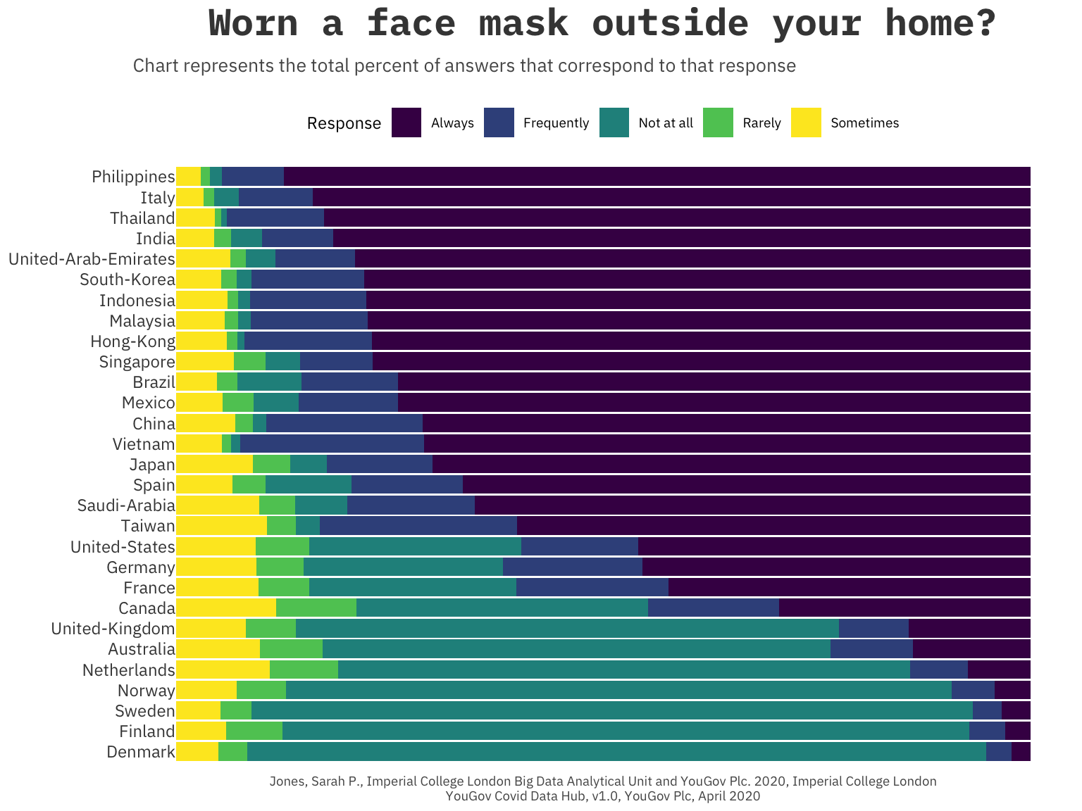

#trasnport
covid_data %>%
  filter(variable == 'transport',
         Response != ' ') %>%
  ggplot(., aes(x = reorder(country,order), y = n, fill = Response)) + 
  geom_bar(position = "fill", stat = "identity") +
  coord_flip() +
  scale_fill_viridis(discrete = TRUE, option = 'C') +
  a_plex_theme(grid = FALSE) +
  theme(legend.position = 'top',
        axis.text.x = element_blank(),
        plot.title = element_text(hjust=0.5),
        axis.text.y = element_text(margin = margin(t=0,r=-25,b=0,l=0)),
        plot.caption = element_text(hjust = 0.5,size = 7)) +
  labs(title='Avoid taking public transport?',
       subtitle='Chart represents the total percent of answers that correspond to that response',
       x=NULL,
       y=NULL,
       caption='Jones, Sarah P., Imperial College London Big Data Analytical Unit and YouGov Plc. 2020, Imperial College London\nYouGov Covid Data Hub, v1.0, YouGov Plc, April 2020')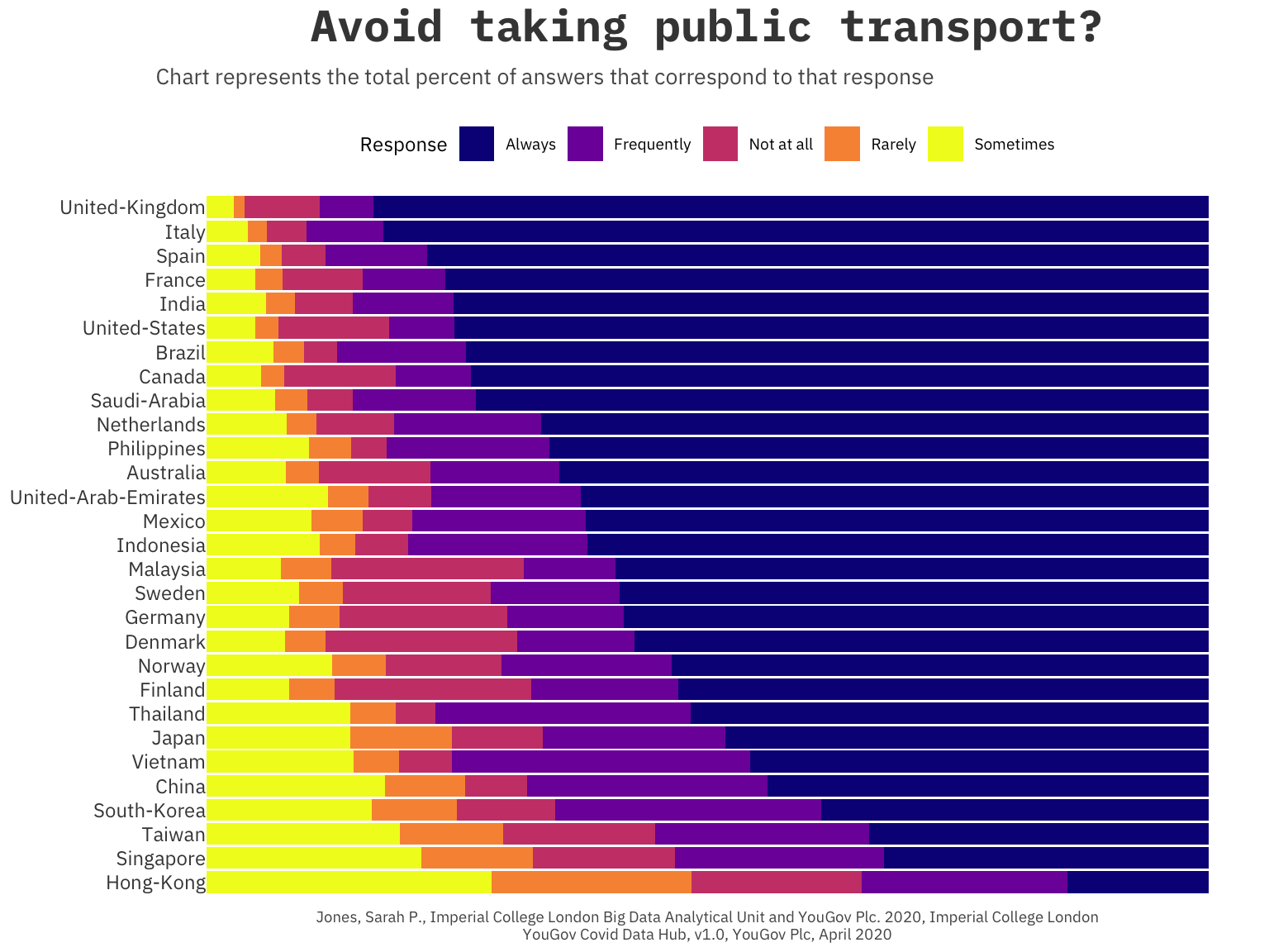

#gathering
covid_data %>%
  filter(variable == 'gathering',
         Response != ' ') %>%
  ggplot(., aes(x = reorder(country,order), y = n, fill = Response)) + 
  geom_bar(position = "fill", stat = "identity") +
  coord_flip() +
  scale_fill_viridis(discrete = TRUE,option = 'B') +
  a_plex_theme(grid=FALSE) +
  theme(legend.position = 'top',
        axis.text.x = element_blank(),
        plot.title = element_text(hjust=0.5),
        plot.subtitle = element_text(hjust=0.5),
        axis.text.y = element_text(margin = margin(t=0,r=-25,b=0,l=0)),
        plot.caption = element_text(hjust = 0.5,size = 7)) +
  labs(title='Avoid small social gatherings?',
       subtitle='No more than two individuals\nChart represents the total percent of answers that correspond to that response',
       x=NULL,
       y=NULL,
       caption='Jones, Sarah P., Imperial College London Big Data Analytical Unit and YouGov Plc. 2020, Imperial College London\nYouGov Covid Data Hub, v1.0, YouGov Plc, April 2020')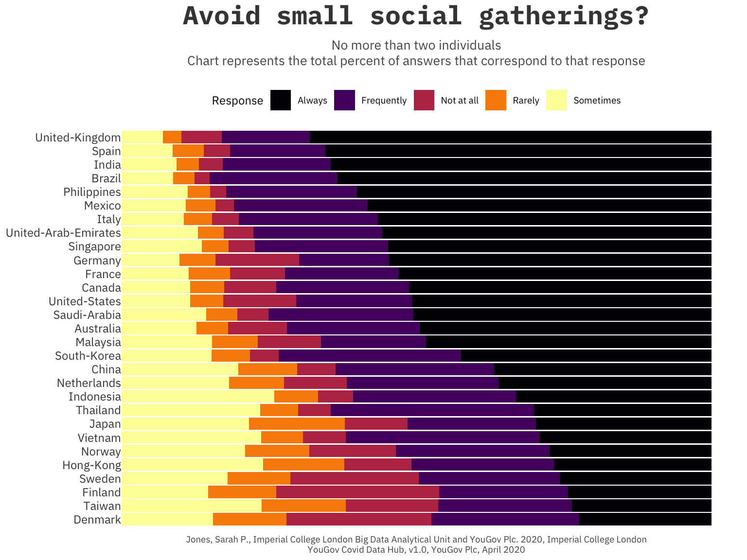

Some initial thoughts are on some specific countries that seem to vary in responses. The United Kingdom jumps out as ranking highly in ‘Always’ responses for avoiding public transit and small social gatherings but low for wearing face masks. I do not know enough about the laws around Covid 19 in the UK but these sorts of patterns are what I hope to investigate.