Number one you should join me (and all other great friends of the pod) and listen to their podcast. Number two is that I did not want to sit idly by and be apathetic, I wanted to learn and know how this was happening. I have read we as a team are improving, and to trust the system and that there is a plan but those are all words we have heard before. So I decided to look into the numbers. How are we really doing?

Before I start I want to say that this may come off as condemning of Berhalter. There are a number of internal issues with our soccer federation that I both cannot and do not understand. But what I do believe is that the team’s performance on the field starts and stops with him, so that is what I will try to keep the scope of this to. So first off let’s take a look at the last few manager’s and their win/loss/draws to see how the last couple compare.

library(tidyverse)
library(rvest)
library(awtools)

#look at managers
managers<-read_html('https://en.wikipedia.org/wiki/List_of_United_States_men%27s_national_soccer_team_managers') %>%
  html_nodes('.wikitable') %>%
  html_table() %>%
  data.frame()

managers_clean <- managers %>%
  select(1:7) %>%
  mutate(order=row_number(),
         Managers=gsub('\\s*\\[[^\\)]+\\]','',Managers)) %>%
  group_by(Managers,Years,M,Result..,order) %>%
  gather(type,n,4:6) %>%
  ungroup() %>%
  filter(order<=12)

I pulled the manager information from Wikipedia’s List of USMNT Managers. Once we have that in we create the managers_clean object where we create the order and column data to compare. Then plot.

ggplot(managers_clean,aes(x=reorder(gsub(' ','\n', Managers),order),y=n,fill=type)) +
  geom_bar(position='fill', stat='identity') +
  a_flat_fill() +
  a_plex_theme(grid = FALSE,axis_text_size = 8) +
  scale_x_discrete(position = "top") +
  scale_y_continuous(labels = scales::percent) +
  theme(legend.position = 'top') +
  labs(y='%',
       x='',
       title= 'U.S. Men\'s National Team\nManagers',
       subtitle = 'Win, Loss, and Draw statistics for the last 12 USMNT managers.',
       caption='USMNT Managers List\nfrom Wikipedia',
       fill='')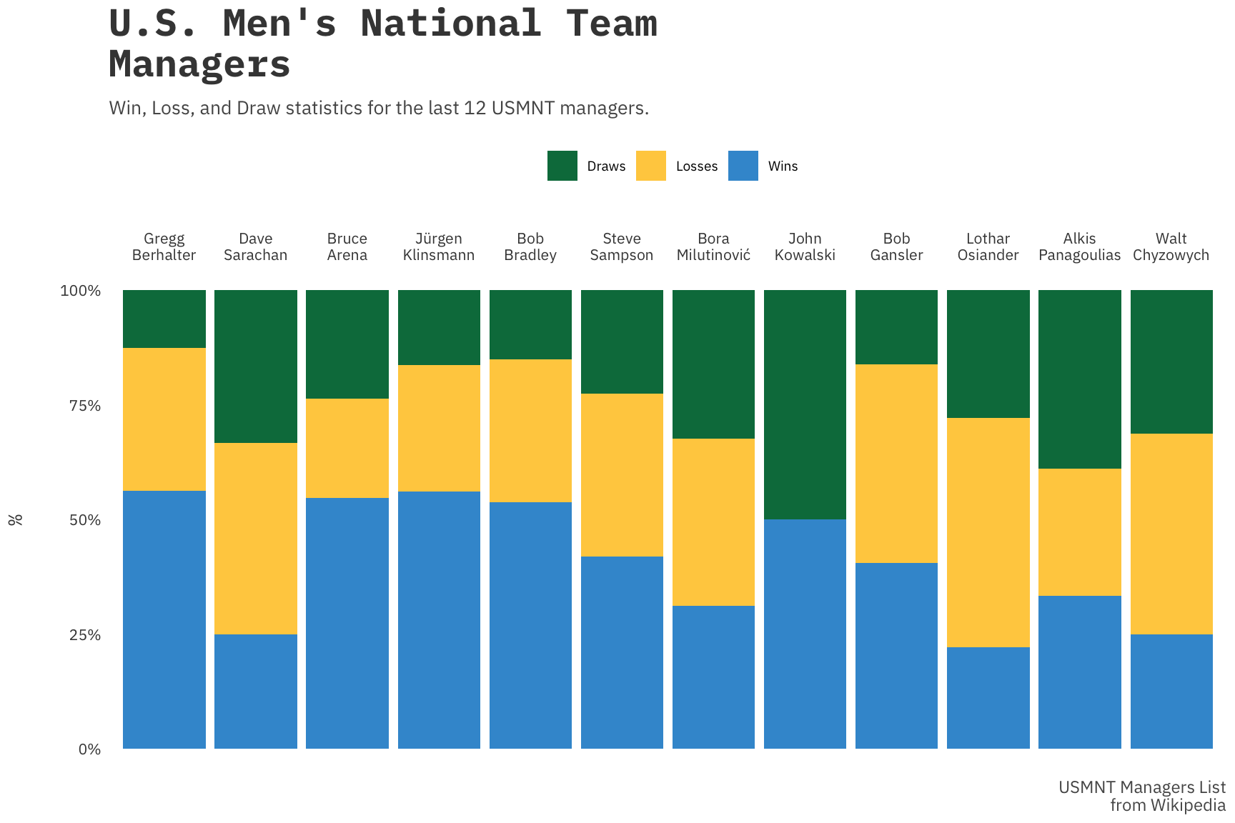

Interesting. Berhalter’s win percentage is one of the highest at ~60%, so maybe we really are doing alright. One thing this sort of visual does not describe is when these wins happened so I decided to create a list of the last 100 USMNT games which is available in my Dataset-list repo on github. In the last 100 games for the USMNT there were only four total managers.

#load
us_results<-read.csv('https://raw.githubusercontent.com/awhstin/Dataset-List/master/us_results.csv',stringsAsFactors = FALSE)

us_results<-us_results %>%
  mutate(trend=if_else(result == 'W',1,0),
         trend.winloss=case_when(result=='W'~1,result=='T'~0,result=='L'~-1)) %>%
  group_by(manager) %>%
  mutate(game=1:n()) %>% ungroup()

#summary
trends <- us_results %>%
  group_by(manager) %>%
  mutate(trend=cumsum(trend),
            trend.winlosst=cumsum(trend.winloss))

overall <- us_results %>%
  arrange(order) %>%
  mutate(trends=cumsum(trend.winloss))

Once the game data is loaded in we create two new variables, trend and trend.winloss. The first of these helps us paint the picture of how the managers compare to each other with wins by calculating a running sum of wins which we will plot by game.

ggplot(trends,aes(x=game,y=trend,color=manager,group=manager))+
  geom_point() +
  geom_line() +
  a_flat_color() +
  a_plex_theme() +
  labs(x='Game',
       y='Wins')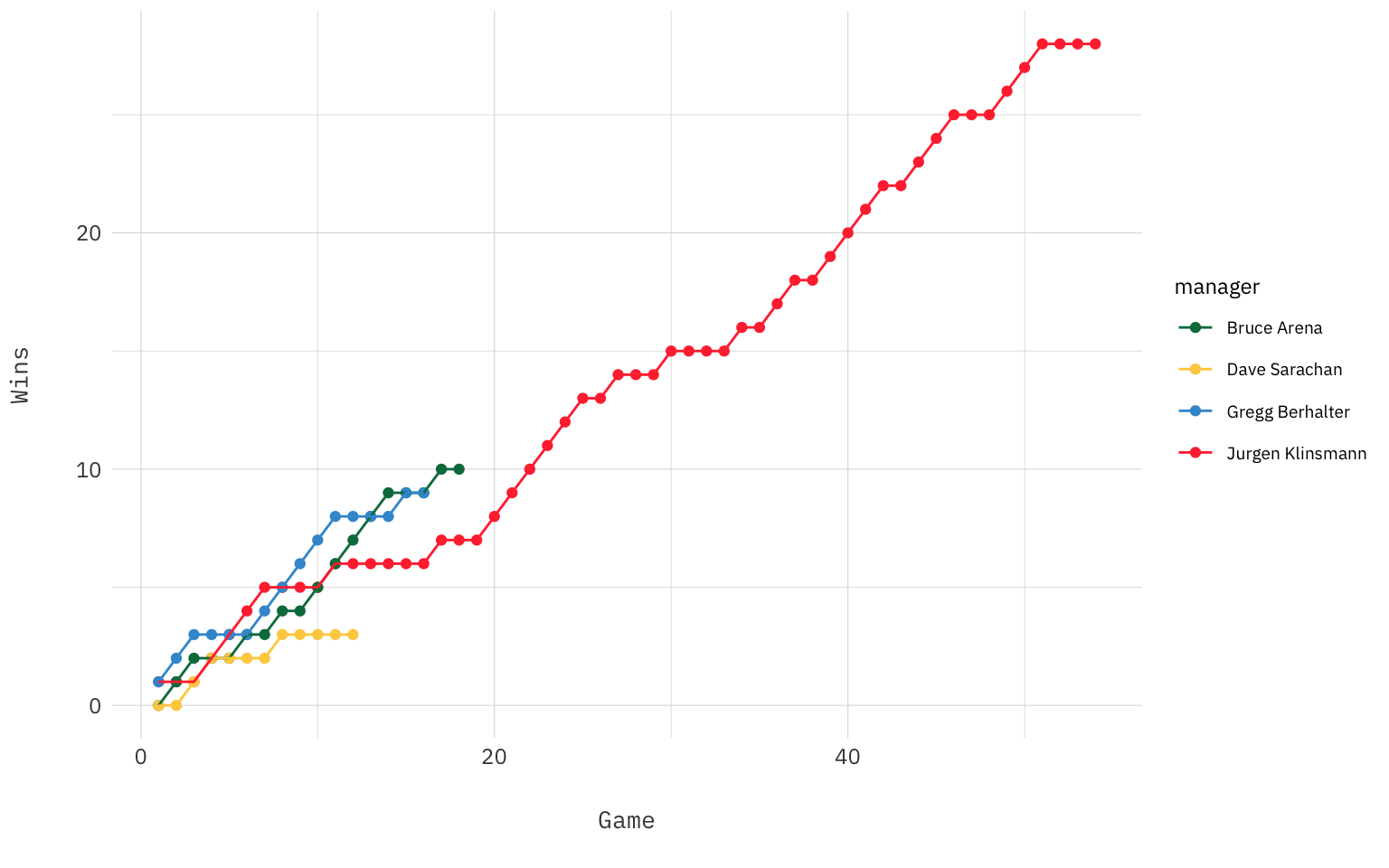

So it looks like Berhalter has had a pretty decent start compared to the last few managers but we can see a recent string of draws/losses that have brought him back in line with the others. As we can see it took quite a few games before Jurgen’s team hit its stride. So in terms of number of wins it looks like Berhalter is certainly performing within the expected range. This visualization though is just looking a wins, we need to incorporate all the games to get the full picture.

Another way to look at this then is with the trend.winloss which we change the calculation slightly to +1 for a win, 0 for a draw, and -1 for a loss. This will help us see the bigger picture of how the USMNT is currently trending.

ggplot(overall,aes(x=order,y=trends,color=manager))+
  geom_point(alpha=.5) +
  geom_line(size=1.5) +
  a_flat_color() +
  a_plex_theme() +
  theme(legend.position = 'top') +
  labs(
    x='Game',
    y='Trend',
    title='USMNT Last 100 Games',
    subtitle='USMNT win-loss trend over the last 100 games by manager',
    caption='Interim Manager: Dave Sarachan',
    color=''
  )

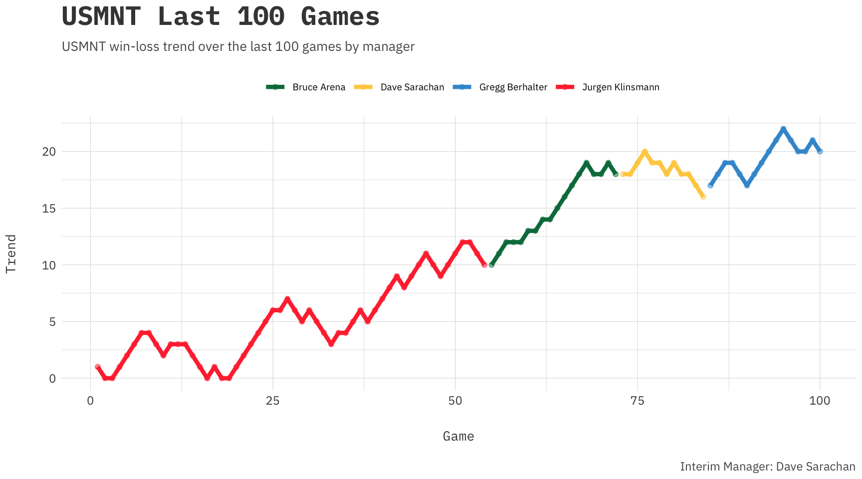
This paints the picture that I have in my mind. As you can see the trend of the USMNT over the last few games is in decline and the losses have made Berhalter’s start less than ideal. With 9 wins in 16 matches, as the first chart shows, is a good return. But those wins were mostly strung together and only one win in the last five is certainly not promising. Two of those losses came at the hands of a good Mexico team but poor defense and lackluster creation on offense seem to be in the lineup for the US recently. I do have hope that this is merely a blip like so many other blips (even in the last 100 games) but with press like this it can be hard:

• There’s no reason to believe this USMNT will ever get good
• Christian Pulisic and the USMNT slump to nightmare defeat vs. Canada | CONCACAF Nations League
• Alexi Lalas: Time has come for USMNT to ‘say goodbye to romance’

Our next two fixtures are Canada and Cuba again in the CONCACAF Nations League so I hope these will be two opportunities to reverse this trend.